Guide to Keras Image Classification Model using CNN

The process of image classification assigns classes to an entire image. Images are anticipated to have just one class per image. Mastering Keras and CNNs have revolutionized image classification tasks.

Let’s dive into the world of Keras and CNNs and take your image recognition skills to the next level. You will perform image classification using neural networks to extract features from images and classify them based on these features with hands-on examples.

Creating a Neural Network with Keras

A simple neural network typically looks like the one shown below:

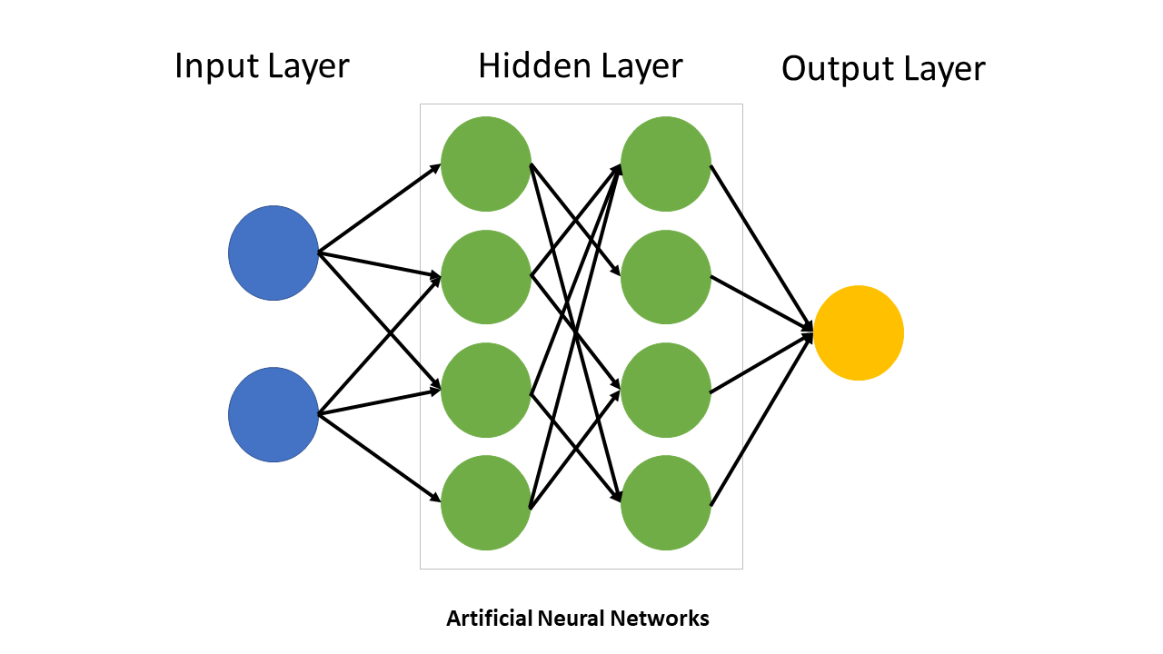
Machine learning includes convolutional neural networks, also known as convents or CNNs. It is a subset of several artificial neural network models employed for diverse purposes and data sets. A convolutional neural network is most often applied to image processing problems.

In a regular neural network, the neurons are connected to every other neuron; in a CNN, neurons are connected to neurons close to it, and all have the same weight. A CNN is made up of a convolutional layer and a pooling layer. However, like other neural networks, it can have RELU and fully connected layers. A convolutional layer is mostly used to detect patterns using filters.

Keras

Keras is a high-level deep learning API written in Python for neural networks. It supports multiple backend neural network computations and makes implementing neural networks easy. Keras empowers engineers and researchers to take full advantage of its cross-platform capabilities of TensorFlow too. Keras provides a Python interface for artificial neural networks.

Keras is a high-level interface that uses Tensorflow for its backend and supports almost all the models of a neural network. Keras is incredibly expressive, flexible, and appt for innovative research. It is a powerful, open-source, open-source API for developing complex deep-learning models. It wraps efficient numerical computational libraries Theano and TensorFlow and allows you to define and train neural networks in a few lines of code.

The following steps are involved in building a model in Keras.

• Define a network
• Compile Network
• Fit Network
• Evaluate Network
• Make predictions

Steps To build an image classification model

Step 1: Load the data

I will be using a dataset from the library called “datasets” that allows us to download the dataset from the server easily, and there will be no need to download the dataset on your computer. In this example, we are loading the fashion mnist dataset that consists of a training set with 60,000 examples and a test set with 10,000 examples. It consists of 10 classes, each a grayscale image with size 28*28.

Let us now load this dataset after importing the TensorFlow and Keras.

#import the required libraries

import tensorflow as tf

from tensorflow.keras import datasets, layers, models

#load the dataset

(x_train, y_train), (x_test, y_test) = tf.keras.datasets.fashion_mnist.load_data()

Step 2: Analyze the data

Let’s look at the shape of x_train and x_test

print('Training data shape : ', x_train.shape, y_train.shape)

print('Testing data shape : ', x_test.shape, y_test.shape)

Training data shape : (60000, 28, 28) (60000,)
Testing data shape : (10000, 28, 28) (10000,)

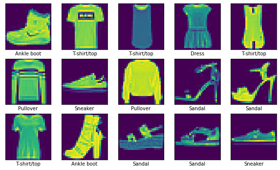
Next, we will display a few images to verify if the dataset looks correct.

class_names =["T-shirt/top","Trouser","Pullover","Dress","Coat","Sandal","Shirt","Sneaker","Bag","Ankle boot"]

plt.figure(figsize=(10,10))
for i in range(15):
    plt.subplot(5,5,i+1)
    plt.xticks([])
    plt.yticks([])
    plt.grid(False)
    plt.imshow(x_train[i])
    plt.xlabel(class_names[y_train[i]])
plt.show()

Step 3: Preprocess the data

Let’s reshape the data to a matrix of size 28281 and then normalize it using the below code.

x_train=x_train.reshape(-1,28,28,1)
x_test=x_test.reshape(-1,28,28,1)
x_train=x_train/255.0
x_test=x_test/255.0

Step 4: Creating the model

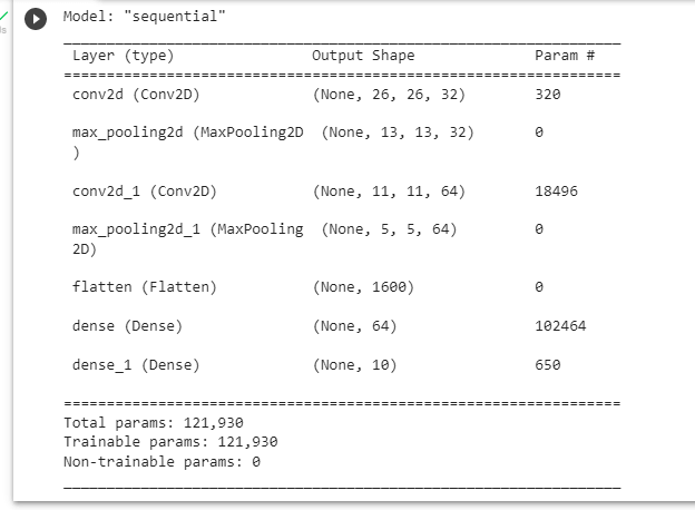
As we have discussed, a CNN consists of convolutional and MaxPooling layers. So, we are adding 2 convolutional layers followed by 2 MaxPooling layers. We then use the Flatten layer that converts the 3D output tensor to 1D. Finally, we add 2 dense layers by specifying the activation function as “softmax” for the last layer.

cnn=models.Sequential([

    layers.Conv2D(filters=32, kernel_size=(3,3), input_shape=(28,28,1), activation="relu"),

    layers.MaxPooling2D((2,2)),

    layers.Conv2D(filters=64, kernel_size=(3,3), activation="relu"),

    layers.MaxPooling2D((2,2)),

    layers.Flatten(),

    layers.Dense(64, activation="relu"),

    layers.Dense(10, activation="softmax")
])

Step 5: Compile the Model

Now that we have successfully created the model, the next step would be to compile the model. We are using the optimizer as adam and the loss function as sparse_categorial_crossentropy and specifying accuracy as the metrics.

cnn.compile(optimizer='adam',

    loss='sparse_categorical_crossentropy',

    metrics=['accuracy'])

To view the summary of the model, use:

cnn.summary()

Step 7: Train the model

The main step is training the model using the function fit() function. We are specifying epochs as 10. The fit function returns a history object which we will use further to plot the accuracy and loss metrics.

history=cnn.fit(x_train,y_train,epochs=10,
    validation_data=(x_test,y_test))

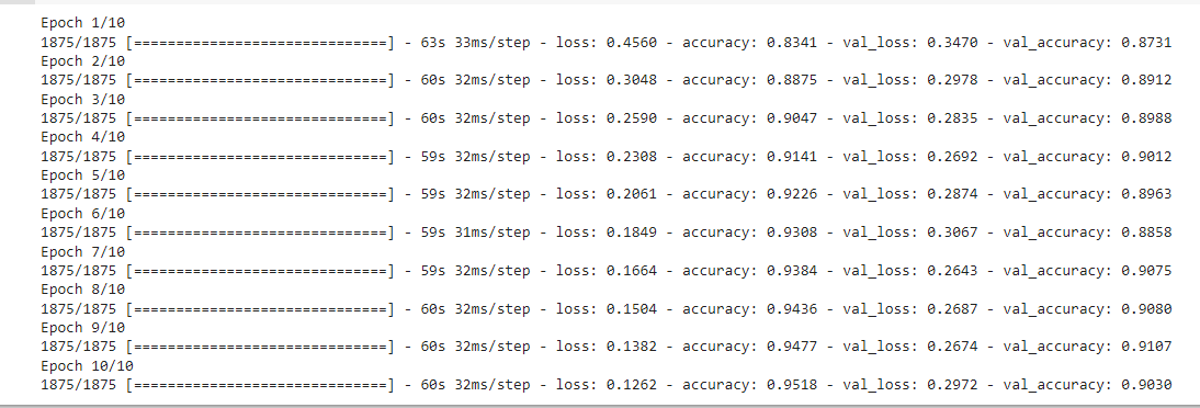
Finally, after training the model for 10 epochs, we can observe that the training accuracy is 90% which is quite good with this dataset.

Step 7: Evaluate the model

test_loss, test_acc = cnn.evaluate(x_test,y_test, verbose=2)

313/313 - 3s - loss: 0.2972 - accuracy: 0.9030 - 3s/epoch - 9ms/step

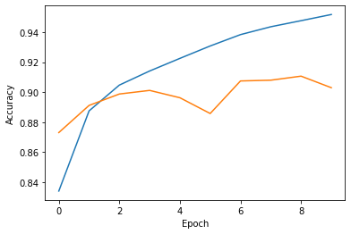
The test accuracy is 90.30% which is quite impressive, and a loss of 0.2972 is not bad. Let us now move further and plot the accuracy and loss between training and validation data.

plt.plot(history.history['accuracy'], label='accuracy')

plt.plot(history.history['val_accuracy'], label='val_accuracy')

plt.xlabel('Epoch')

plt.ylabel('Accuracy')

Conclusion

In this article, we have created an image classification model using convolutional neural networks on the fashion mnist dataset. We have covered the step-by-step procedure along with the code examples. Finally, we have observed that the accuracy was 90% which is quite good.